 |
 |
 |
 |
| Home | Technology | Products | Contact us |
|
|
|
1. Transit-time Technology
A typical transit-time ultrasonic flow meter system utilizes two transducers that function as both ultrasonic transmitter and receiver. The flow meter operates by alternately transmitting and receiving a burst of sound energy between the two transducers and measuring the transit time that it takes for sound to travel between the two transducers. The difference in the transit time measured is directly and exactly related to the velocity of the liquid in the pipe. For detailed explanations, please click here. 2. Ultrasonic Doppler Technology
Two ultrasonic transducers are employed in the system. One transmits a continuous ultrasonic wave into the flow. Another one is used to receive the ultrasonic wave back scattered from suspending particles (or targets). The received wave has a frequency shift comparing with the transmitted one. This shift is the so-called Doppler frequency shift, proportional to the flow velocity. Therefore, by detecting the Doppler frequency, we are able to derive the flow velocity. The flow rate of a pipe flow is then obtained by computing the product of the velocity and the cross-section area of the pipe. 3. Cross-Correlation Measurement Technology
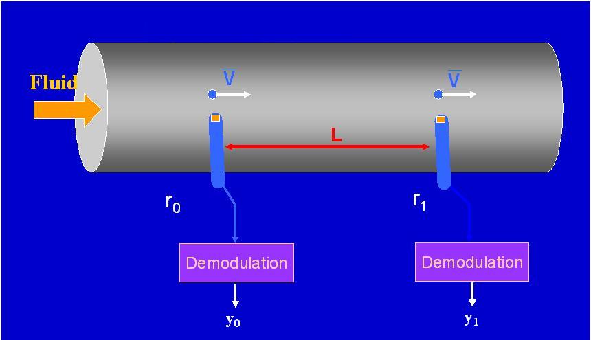
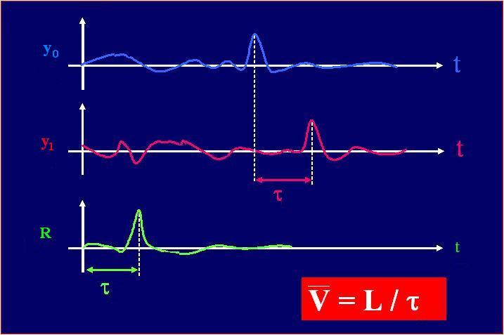
A turbulent flow has a cascade structure of eddies. Along the flow, the characteristics of those structures do not change much within a certain distance, the so-called Correlation Length. In other words, turbulence at a certain distance apart are correlated. Based on this assumption, we can place two pairs of ultrasonic sensors along the flow direction to pick up the turbulence signature. Obviously, the upstream sensor will detect a flow signature L/V seconds earlier than the downstream one, where L is the space between the two sensors and V is the flow velocity. By comparing the signals from the two sensors, we are able to determine the time delay, thus, to calculate the velocity.
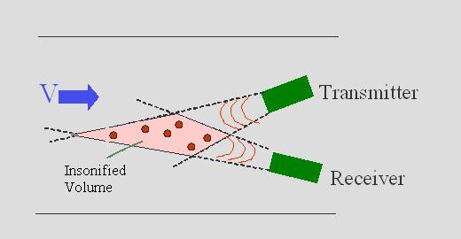
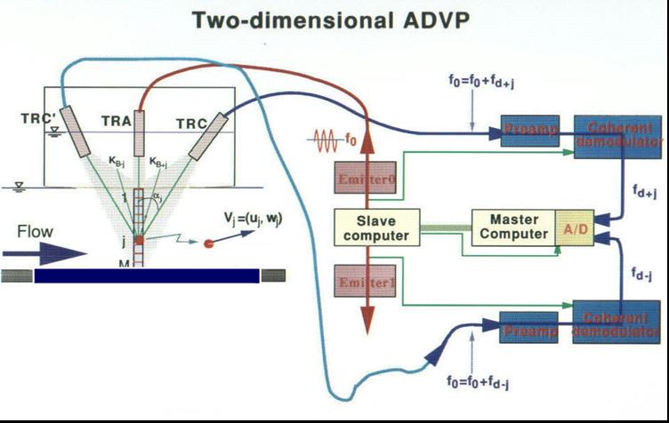
4. Acoustic Doppler Velocity Profiling Technology
Three acoustic transducers are installed as shown in the figure. The center one is usually a narrow-beam transducer. It transmits a burst of sound pulses with a certain Pulse Repetition Frequency (PRF). The other two are large angle transducers. They receive the ultrasonic wave scattered from suspending particles (or targets) of the water column
insonified by the transmitting and receiving sound beams. By using pulse-to-pulse algorithm, we are able to obtain the Doppler frequency shift at two directions, from which a 2D velocity profile is formed.
Click
here
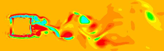
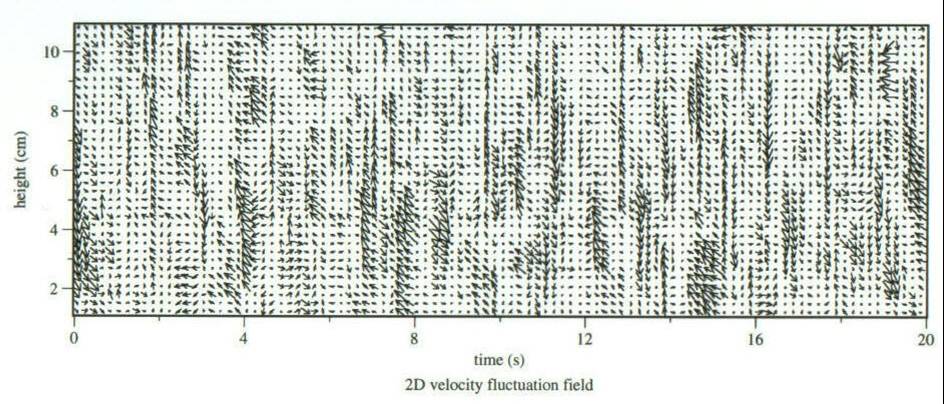
to see an example of 2D velocity profiles obtained in a laboratory open-channel flow. |
|||||||||
|